With the Functor-Applicative-Monad proposal just around the corner, I’ve been wondering what exactly the relation between Applicative and Monad is. Every Monad can be made a Functor with fmap = liftM where
liftM :: Monad m => (a -> b) -> m a -> m b
liftM f ma = do a <- ma
                return (f a)
In fact, parametricity guarantees that fmap = liftM; it’s a free theorem. There is another law relating Functor and Monad, ma >>= f = join (fmap f ma). This law is particularly interesting because if you define a Monad the way mathematicians do using join instead of (>>=) then you must have Functor as a superclass in order to define (>>=). So it seems very natural for Functor to be a superclass of Monad.
However, it’s not so obvious to me why Applicative should be a superclass of Monad. It’s true that every Monad can be made an Applicative with (<*>) = ap where
ap :: Monad m => m (a -> b) -> m a -> m b
ap mf ma = do a <- ma
              f <- mf
              return (f a)
One should naturally expect that (<*>) = ap is a law when Applicative is a superclass of Monad. But, (<*>), unlike fmap, is not uniquely determined. A type constructor may have more than one instance. For example, lists have two useful instances.
ap :: [a -> b] -> [a] -> [b]
ap fs as = [f a | a <- as, f <- fs]

zap :: [a -> b] -> [a] -> [b]
zap [] _ = []
zap _ [] = []
zap (f:fs) (a:as) = (f a) : zap fs as
ap delivers a list of all functions in the first list applied to all values in the second list while zap goes down the lists applying functions to values at the same index. So which do you choose? Well, ap is the one which is compatible with the Monad instance on lists, so it wins. zap is used as the Applicative instance for a newtype on lists, the ZipList. Interestingly, there is no compatible Monad instance on ZipLists.
The ambiguity for lists resolves nicely enough. But in creating data types for concurrency, one runs into cases where you might want Applicative and Monad instances where (<*>) /= ap. A really good example can be found in the Haxl paper. Haxl is a library developed by Facebook to manage data requests in a way to maximize concurrency for the sake of efficiency. In section 4 of the paper, we find out that for the type constructor Fetch,
Blocked (Done (+1)) <*> Blocked (Done 1) = Blocked (Done 2)
Blocked (Done (+1)) `ap` Blocked (Done 1) = Blocked (Blocked (Done 2))
I won’t go over the details here but the takeaway is that the Applicative can take advantage of looking at both arguments of (<*>) which are both in Fetch while the Monad cannot because it must use (>>=) the second argument of which is a function with pure input. So here we have an example of a law breaking Applicative/Monad. As with ZipList, there is no Monad instance which is compatible with the Applicative instance. So why not newtype? The motivation is that we want to be able to use concurrencly implicitly without the overhead of having to wrap and unwrap a newtype. Whether that justifies breaking the law is a judgment call. Notice however that the law breaks in a well defined way, that is (<*>) is equal to ap up to idempotency of Block, the relation that Block . Block = Block .
I want to work through another example that was inspired by concurrency in Purescript.
First lets take care of the imports.
import Control.Applicative
import Control.Concurrent
import Control.Concurrent.Async
import Control.Concurrent.MVar
import Control.Monad.IO.Class
import Data.Traversable
import Prelude hiding (mapM)
import System.Random
Annoyingly we have to hide either the mapM from Prelude or Data.Traversable but this should be fixed by the Foldable/Traversable in Prelude proposal. The type constructor we’ll work with is for callbacks.
newtype Callback a = Callback {runCallback :: (a -> IO ()) -> IO ()}
You should recognize that Callback is isomorphic to ContT () IO, so we can just crib the definitions of Functor and Monad instances from your favorite source. We’ll also give a MonadIO instance.
instance Functor Callback where
    fmap f c = Callback (\k -> runCallback c (k . f))

instance Monad Callback where
    return a = Callback (\k -> k a)
    c >>= f = Callback (\k -> runCallback c (\a -> runCallback (f a) k))

instance MonadIO Callback where
    liftIO io = Callback (\k -> io >>= k)
For the Applicative instance we want to take advantage of the ability to do our IO side effects concurrently. Let’s see how this works.
instance Applicative Callback where
    pure a = Callback (\k -> k a)
    cf <*> ca = Callback $ \k -> do
        vf <- newEmptyMVar
        va <- newEmptyMVar
        let finish = do f <- takeMVar vf
                        a <- takeMVar va
                        k (f a)
        race_ (runCallback cf (putMVar vf) >> finish)
              (runCallback ca (putMVar va) >> finish)
Ok, so what’s going on the definition of (<*>)? Well first we create new empty mutable variables in which we will store a function f and a value a to apply it to, but which we must perform some IO effects to get. finish is where we perform the callback on the result. finish looks a whole lot like ap. The magic happens in the function race_ which is from Simon Marlow’s delightful async package. It runs two IO actions concurrently, canceling the loser. Because finish blocks when either vf or va are empty, both callbacks are run concurrently with a putMVar as the callback, filling up the variables. Then finish will unblock and the first branch to complete it wins the race.
Let’s see the difference in performance between the Applicative and Monad instances on an example.
square :: Int -> Callback Int
square n = do liftIO $ do let second = 10^6
                          random <- randomRIO (0 , second)
                          threadDelay random
                          let time = fromIntegral random / fromIntegral second
                          putStrLn $ "Squaring "
                              ++ show n ++ " after "
                              ++ show time ++ " seconds."
              return (n^2)

main = do putStrLn "Traversing [1..10] using Monad"
          runCallback (mapM square [1..10]) print
          putStrLn "Traversing [1..10] using Applicative"
          runCallback (traverse square [1..10]) print
And here’s an example of what the output looks like.
Traversing [1..10] using Monad
Squaring 1 after 0.723773 seconds.
Squaring 2 after 0.603614 seconds.
Squaring 3 after 0.203097 seconds.
Squaring 4 after 0.535666 seconds.
Squaring 5 after 0.414605 seconds.
Squaring 6 after 0.807218 seconds.
Squaring 7 after 0.580662 seconds.
Squaring 8 after 0.715894 seconds.
Squaring 9 after 0.641902 seconds.
Squaring 10 after 0.180422 seconds.
[1,4,9,16,25,36,49,64,81,100]
Traversing [1..10] using Applicative
Squaring 4 after 4.8804e-2 seconds.
Squaring 5 after 0.140811 seconds.
Squaring 3 after 0.142185 seconds.
Squaring 7 after 0.373733 seconds.
Squaring 9 after 0.386626 seconds.
Squaring 8 after 0.393645 seconds.
Squaring 1 after 0.417399 seconds.
Squaring 6 after 0.780407 seconds.
Squaring 2 after 0.803894 seconds.
Squaring 10 after 0.96637 seconds.
[1,4,9,16,25,36,49,64,81,100]
The Monad is forced to perform the effects consecutively, taking up to 10 seconds (ignoring the time it takes to get a random number and to print). The Applicative performs the effects concurrently, taking only up to 1 second. So here’s another example where (<*>) /= ap and we may be somewhat justified by the desire for implicit concurrency. Notice that it’s just the effects that are different, not the result. Said another way, if we bind x <- mf <*> ma and y <- mf `ap` ma then we have that x = y so we’re breaking the law but not flagrantly.

 and mod out by the circle relation:


 .
. the space
  of endomorphisms of
  , forms an algebra where our multiplication is composition of linear maps and our unit is the identity map
  .
.  which preserves multiplication and unit.
 called comultiplication, counit which are coassociative, and counital where
  is the field of scalars. This guarantees that the category
  of finite dimensional representations of
 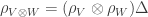 and
and  . We also require a map
  called the antipode which switches the order of multiplication and is the convolution inverse to the identity. This guarantees that
  .
. such that
  is a braiding, where
  is the swap map
  and where
  is a twist, then we call
  and the result is a ribbon Hopf algebra. This discovery led to a whole slew of new invariants and a new understanding of old invariants. For instance the Jones’ polynomial and the Kauffman bracket are related to the quantization of the most basic Lie algebra
  . Invariants of tangles derived from quantized Lie algebras are called Reshetikhin-Turaev invariants or simply quantum invariants. When applied to links they give polynomials in a variable
  .
. along with a class (for technical reasons a class, not a set) of morphisms
  . Each morphism has a source object and a target object so that we can think of a morphism as an arrow
  . There is a composition operation of morphisms
  which is defined only if the source of
  is the target of
  . There is also an identity morphism
  for every object
  and unital
  .
.
 of linear maps from
  and evaluates to the scalar
  . Coevaluation makes use of the isomorphism
  where
where 

 -bundle
  with a connection
  with curvature
  .
. is just the set of imaginary numbers
  with trivial Lie bracket
 ![{[},{]}=0](https://s0.wp.com/latex.php?latex=%7B%5B%7D%2C%7B%5D%7D%3D0&bg=ffffff&fg=333333&s=0&c=20201002) . The local potential is a real-valued 1-form
. The local potential is a real-valued 1-form  defined by
  . The local field strength
  is defined by
  .
. with
with  . We see that local connections are related by
  , so that local potentials are related by
  . Local curvatures are related by
  , so that local field strengths are related by
  . This means that the field strength is globally defined on
  .
. so
so  , so the homogeneous Maxwell equation comes along for free. We can get the inhomogeneous Maxwell equation by requiring that
  .
. given by multiplication
  . Associated to our principal
  locally given by
  . We will write sections of the associated bundle as
  . We can define the d’Alembert operator
  . If we require the Klein-Gordon equation,
  , then we have a theory of a charged spin-0 particle coupled to electromagnetism.
 , i.e. matrices
  such that
  where
where  , or equivalently
  for any events
  in Minkowski spacetime. This group has 4 connected components coming from
  and
and  or
or  . The component containing the identity is called the proper, orthochronous Lorentz group
  . Physically it contains all rotations, and boosts (Lorentz tranformations) and so
  .
. by the simply connected group
  , i.e.
  complex matrices
  . First we identify Minkowski spacetime
  with the space of
  such that
  , in such a way that if
  then
then  . Then we can define a covering map
  by identifying
  with
with  . We have that
  since
since . It can be shown that
  is a 2-1 homomorphism of Lie groups.
 , the “spin
  ” representations given by multiplication
  and multiplication by the adjoint
  . The Dirac representation is the direct sum of these representations
  .
. be the orthonormal frame bundle for spacetime. Its fibers
  are ordered orthonormal bases of
  , or equivalently isometries
  . There is a right action of
  which makes the frame bundle an
  has 4 components and a choice of component
  is a space and time orientation. Then the restriction
  is an
is an  on
on  . The torsion of a connection
  on
on  . It turns out that there is a unique connection whose torsion is
  . This is the Levi-Civita connection
  and a smooth map
  such that
  is an
is an  . We can define a connection
  on
on  where
where  is the isomorphism of Lie algebras induced by
  such that
  , i.e. the Dirac operator is the “square root” of the d’Alembert operator. A full understanding of the Dirac operator requires
  . It turns out that the smallest representation
  of this Clifford algebra is 4-dimensional which is why we need a 4-dimensional representation of
  where
where 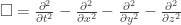 , define

 . This gives us a theory of a spin-
 . In order to couple to the electromagnetic field, we will rather think of the electron taking its values in a representation of the charged spin group
  .
. -bundle
  with a
  -bundle
  . Define
  and
and  . This is a
  -bundle with
  . Given connections
  on
on  , we can define a connection
  by
by  with
with  given by
  .
. on
on  given by combining the Dirac representation with multiplication by
  . This structure is
  -invariant so defines a
  -bundle. We get an associated vector bundle with an associated connection and Dirac operator
![\partial_{[\lambda}F_{\mu\nu]}=0](https://s0.wp.com/latex.php?latex=%5Cpartial_%7B%5B%5Clambda%7DF_%7B%5Cmu%5Cnu%5D%7D%3D0&bg=ffffff&fg=333333&s=0&c=20201002)
 we can define a 2-form
  . We can also define a 1-form
  . Then we can re-express Maxwell’s equations using exterior differentiation and the
  then follows from the inhomogeneous Maxwell equation. We expect from the homogeneous Maxwell equation that
  . In fact this is only true locally. This means that for every event
  in our spacetime
  with
with  and a 1-form
  on
on  . This follows from
  , the area form of the unit sphere in spherical coordinates, then
  since
since  by antisymmetry of wedge product of 1-forms. Also, taking
  to be the unit sphere, we know that
  . However, by
  . So, we cannot have
  and worldline, the time axis,
  . Mathematically, what is happening is that the complement of the time axis has nontrivial topology. Specifically its second
  . We would like to find a global mathematical object corresponding to the potential which doesn’t depend on our “choice of gauge”. This is our motivation for understanding connections on principal bundles.
 is a group of matrices. A principal
  of
of  and for any
  there is an open set
  called a “local trivialization” such that
  . Local trivializations correspond to the physical notion of “choice of gauge”.
 .
. with
with  such that
  . It can be shown that there is a canonical 1-1 correspondence between local sections
  and local trivializations
  .
. by
by  where
where  . This is well defined since
  . Transition functions correspond to the physical notion of “change of gauge”. We can relate any two local sections by
  .
. be the Lie algebra for
  and
and  is the tangent field on
  , then
  . Also we require that
  .
. . Local connections are related by
  .
.![\Omega=d\omega+\frac{1}{2}[\omega,\omega]](https://s0.wp.com/latex.php?latex=%5COmega%3Dd%5Comega%2B%5Cfrac%7B1%7D%7B2%7D%5B%5Comega%2C%5Comega%5D&bg=ffffff&fg=333333&s=0&c=20201002) meaning
meaning ![\Omega(X,Y)=d\omega(X,Y)+\frac{1}{2}[\omega(X),\omega(Y)]](https://s0.wp.com/latex.php?latex=%5COmega%28X%2CY%29%3Dd%5Comega%28X%2CY%29%2B%5Cfrac%7B1%7D%7B2%7D%5B%5Comega%28X%29%2C%5Comega%28Y%29%5D&bg=ffffff&fg=333333&s=0&c=20201002) . We can define local curvature by
. We can define local curvature by  . Local curvatures are then related by
  . The Bianchi identity says
 ![d\Omega=[\omega,\Omega]](https://s0.wp.com/latex.php?latex=d%5COmega%3D%5B%5Comega%2C%5COmega%5D&bg=ffffff&fg=333333&s=0&c=20201002) .
.

 in variables
  so that concentrating on a neighborhood of a crossing in a diagram for
 to a link diagram
  . Finally we require a normalization, that for the empty link
  . From this we can deduce that the bracket of
  circles is
  .
.
 and
and  . Solving for
  in terms of
  .
.

 . To calculate it, take a blackboard diagram for the framed link and apply the skein relation, the circle relation and the normalization relation until you reach the answer.
 . Here,
  the total writhe is the sum of signs of all crossings in the diagram and it is this factor which makes
  now invariant under Reidemeister 1 moves.


